Which Direction Is the Target? MIMO and Phased Arrays Made Clear
Start with phase at two receivers, build a two-transmitter/four-receiver virtual array, and distinguish MIMO, beamforming and FMCW.
Contents
Radar from zero — part 6 of 6
Multiple antennas observe an echo at different positions. Their path and phase differences can reveal direction. A phased array applies phase or delay adjustments to favour a direction. MIMO separates transmitter–receiver contributions to obtain more spatial observations. These are related but different concepts.
This lesson connects everyday situations with calculations. Numbers use the stated assumptions.
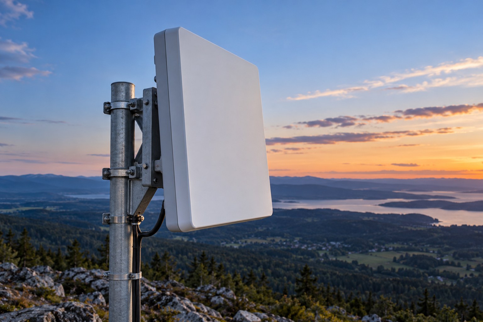
Range alone does not tell you direction
Knowing that a target is three metres away leaves many possible directions at that distance. Direction needs additional information, such as antenna patterns, scanning or spatially separated observations. This lesson focuses on antenna arrays.
An array contains antenna elements at known positions. Its spatial extent is its aperture. Element count matters, but so do placement, wavelength and aperture. Counting channels alone does not establish angular performance.
Two radar ears and a phase difference
Place two receivers a distance d apart on a line. A wave arriving from far away travels slightly different distances to them. Defining θ from broadside, the direction normal to the array, the path difference is approximately d×sin(θ). Thus Δφ≈2πd sin(θ)/λ. The model assumes far-field propagation and known geometry.
At a hypothetical 60 GHz carrier, wavelength is 5 mm. With d=λ/2=2.5 mm and θ=30°, the path difference is 1.25 mm and the phase difference is π/2, or 90°. The angle is measured from broadside, not along the line of elements.
Phased arrays align observations before summing
Suitable phase or delay adjustments can align contributions arriving from one direction before summation. This is beamforming. A transmit array can similarly favour a direction without mechanically turning the panel.
A beam is not a single laser-like line. It has a main-lobe width and sidelobes. Weighting, calibration and element spacing affect the pattern. Across a wide bandwidth, fixed phase is not the same as fixed time delay, so frequency-dependent beam steering can become an issue.
lambda = 5 mm, d = lambda/2, theta = 30 deg
Deltaphi = 2 pi d sin(theta)/lambda = pi/2 = 90 deg
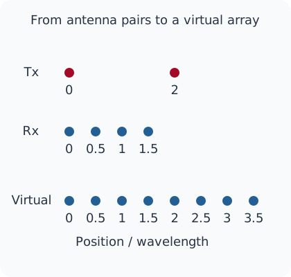
Rx/lambda = [0, 0.5, 1, 1.5]
Tx/lambda = [0, 2]
virtual/lambda = [0, 0.5, 1, 1.5, 2, 2.5, 3, 3.5]
MIMO obtains transmitter–receiver pairs
MIMO means Multiple Input Multiple Output. If the receiver can separate each transmitter’s contribution, each Tx–Rx pair supplies an observation. Separation can use time, frequency or code. Multiplying transmitter and receiver counts gives the number of pairs, not a guarantee of unique virtual positions or improved resolution.
Consider deliberately chosen linear positions: receivers at 0, 0.5λ, 1λ and 1.5λ, transmitters at 0 and 2λ. In the far-field model, adding Tx and Rx positions gives virtual positions. The result is eight positions from 0 to 3.5λ in half-wavelength steps. Positions refer to phase centres; the diagram is not a manufacturable PCB layout.
Eight virtual channels are not eight physical antennas
The example has six physical elements: two transmitters and four receivers. They provide eight distinct pairs. At the hypothetical 60 GHz carrier, the virtual aperture is 3.5λ=17.5 mm. This geometric result is not a promise of angle accuracy or detection range.
Time-division transmitters observe a target at different times. Target motion then contributes phase that can be confused with spatial phase; timing and motion compensation matter. Channel calibration and consistent target association also remain essential.
FMCW and MIMO can work together
FMCW specifies frequency behaviour over time. MIMO supplies spatial channels. Doppler processing can estimate radial velocity. They address different parts of the measurement and are not mutually exclusive menu options.
An educational processing chain uses within-chirp samples for range, across-chirp variation for velocity and spatial-channel differences for angle. Its output can be points containing range, speed and direction. Object classification, tracking and application decisions still require further processing. A radar point alone does not establish identity or an exact object outline.
Turn the application into a numerical requirement
Suppose two objects approximately 3 m away are separated laterally by 0.5 m. Near broadside their angular separation is approximately arctan(0.5/3)=9.46°. This quantifies the question; it does not prove that a chosen sensor can separate them. Angular resolution, noise, actual geometry and unequal reflections need evaluation.
The exercise calculates the 90° phase difference, eight unique virtual positions and the example angle. It does not design an antenna or measure a beam pattern or hardware accuracy. You can now approach a datasheet with four concrete questions: which range, which speeds, what resolution and what field of view are required?
Download the calculation
Run the Python exercise with Python 3.10 or later. It needs no extra libraries, device or network connection. The output below comes from these hypothetical calculations.
phase=90 deg; virtual positions/lambda=[0, 0.5, 1, 1.5, 2, 2.5, 3, 3.5]
virtual aperture=17.5 mm; example angular separation=9.4623 deg
Calculated hypothetical examples only; no hardware, RF or measured-data test.
Primary sources and further reading
The explanation and examples are original editorial teaching material. These primary references support the physical principles and processing models.
Question and answer article
Ask your technical question
Questions and answers are published after moderation. Authors can see their own pending drafts.
No confirmed questions have been registered for this article yet.