How Does Radar See? The Journey of a Returning Wave
Radar measures echoes rather than taking photographs. A wall three metres away introduces delay, distance, speed and angle, then maps the radar families.
Contents
Radar from zero — part 1 of 6
Radar transmits radio waves and receives a small part of their reflection. Comparing the echo with a transmitted reference can reveal distance, radial speed or direction. The available information depends on the waveform, antennas and processing.
This lesson connects everyday situations with calculations. Numbers use the stated assumptions.

The torch analogy: useful, with a limit
Point a torch at a wall. Returning light tells your eyes that the wall is there. Radar also uses reflection, but with radio waves and an electronic receiver. The analogy explains the outward and return paths; it does not mean that an ordinary radar produces a colour photograph or a precise outline. Its output may be a distance, several detected points or only a motion indication.
A target is simply the object whose reflection is being considered: a wall, a car or a water surface. Echo strength depends on material, shape and orientation as well as distance. Two equally distant objects need not produce equally strong signals, and a weak echo does not establish that no object exists.
Three different questions
Range is the direct distance from the radar to the target. Radial velocity is the component of motion that changes that distance. Angle describes a target direction relative to an antenna reference. One measurement does not automatically supply the others. A motion detector need not provide absolute range.
A transmitter generates a signal and an antenna radiates it. The receiver collects the weak echo. A mixer or comparison circuit combines it with a reference; filtering, an analogue-to-digital converter and processing produce useful information. These functions may share one chip rather than occupy separate components.
A three-metre wall and a very short delay
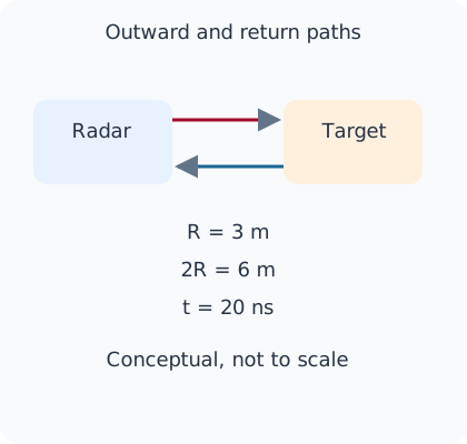
Assume the transmit and receive antennas are approximately co-located and a stationary target is three metres away. The wave travels three metres outward and three metres back: six metres in total. For this calculation, take radio-wave speed in air as approximately 300 million metres per second.
A nanosecond is one billionth of a second. The round trip takes 20 nanoseconds, so R=c×t/2 recovers the range. The factor of two accounts for both legs. This is a monostatic approximation; separated transmitters and receivers require the two path lengths to be considered separately.
R = c t / 2
c = 3.0e8 m/s, R = 3 m
t = 2R/c = 20e-9 s = 20 ns
Why these names do not form one flat list
CW, FMCW, PMCW and FSK describe transmitted-signal behaviour. Simple CW holds frequency constant. FMCW sweeps it, FSK switches among specified frequencies, and PMCW changes phase according to a code. Pulsing describes when transmission is on or off.
Doppler is a physical effect and a way to extract motion from changing frequency or phase; continuous-wave and pulsed systems can both use it. UWB describes very wide bandwidth, not one distance algorithm. MIMO and phased arrays concern multiple antennas and how they are used. A radar can therefore combine FMCW, MIMO and Doppler processing.
Bandwidth, resolution and accuracy
Frequency counts oscillations per second, in hertz. A gigahertz is a billion hertz. Bandwidth describes a frequency span occupied or swept by a signal, not the carrier frequency itself. With appropriate waveforms and processing, wider bandwidth can separate more closely spaced echoes.
Range resolution means distinguishing nearby targets. Accuracy describes closeness to the true range. A radar might track one target repeatably while failing to separate two close targets. A resolution number alone is not the real measurement-error budget.
Your route through the series
This first part is the map. Part two follows a person approaching an automatic door to explain CW and Doppler. Part three calculates how FMCW can measure a car-to-wall gap. Part four introduces FSK and PMCW phase coding. Part five covers pulses, UWB and the difference between radar and two-device ranging. Part six adds multiple antennas and angle.
No module purchase is needed to follow the lessons. The examples and downloadable calculations use stated hypothetical inputs, not RF experiments or measurements from a built device. Covers are disclosed generated illustrations. A real build requires the actual hardware documentation, application constraints and applicable radio rules to be checked separately.
Download the calculation
Run the Python exercise with Python 3.10 or later. It needs no extra libraries, device or network connection. The output below comes from these hypothetical calculations.
R=3 m; round trip=20 ns
Calculated hypothetical examples only; no hardware, RF or measured-data test.
Primary sources and further reading
The explanation and examples are original editorial teaching material. These primary references support the physical principles and processing models.
Question and answer article
Ask your technical question
Questions and answers are published after moderation. Authors can see their own pending drafts.
No confirmed questions have been registered for this article yet.