Oscilloscopes and logic analyzers: reading waveforms and timing
Read voltage waveforms, period and duty cycle. Understand logic thresholds, triggering, sample rate, bandwidth and probe effects with a worked exercise.
Contents
Use an oscilloscope when you need to know how a wire's voltage actually changes. A logic analyzer is useful when the question concerns the order of digital states across several wires and the messages they carry. Troubleshooting a link may require both views: a correctly decoded message does not establish that its electrical waveform is healthy.
Imagine a board issuing a command to turn on a light, with the light sometimes failing to respond. Reading the program is insufficient. When did the command reach the pin, what voltage did it reach, and under what conditions does the receiving device recognize it? Those questions guide this lesson. You do not need to buy an instrument or connect a circuit to follow it.
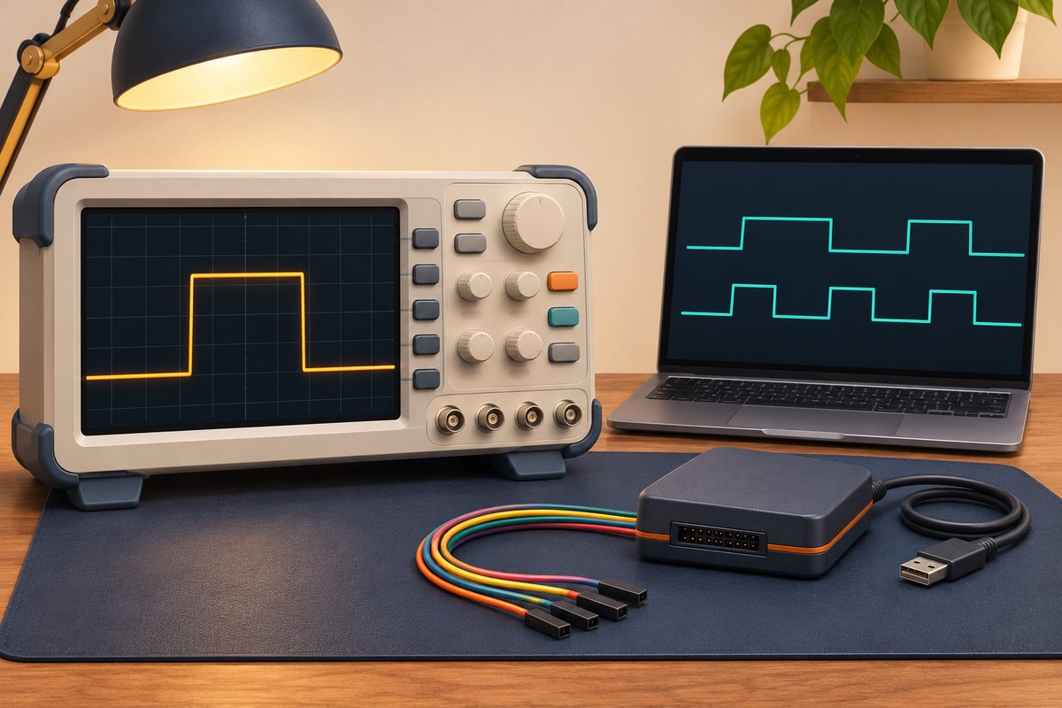
What are a signal and a waveform?
A signal is a changing quantity that carries information or a command. Here that quantity is voltage: electrical potential difference between two points, expressed in volts. Saying a wire is at 3.3 volts is incomplete unless its reference point is understood. All voltages in our examples refer to a hypothetical shared circuit reference.
In the usual voltage-versus-time display, an oscilloscope places time on the horizontal axis and voltage on the vertical axis. The resulting plot is a waveform. A flat upper section means voltage remained approximately steady during that interval. A vertical line in our drawing simplifies a rapid transition; a physical edge takes time and may include ringing or overshoot.
A channel is an instrument's input measurement path. Two channels can capture a command and a response together, such as a controller output and the receiving circuit's supply. This helps establish event order, although events occurring together do not by themselves establish the cause of a failure.
Read a waveform from its axes
The hypothetical output below alternates between zero and 3.3 volts. It is high from zero to 2 milliseconds, low until 5 milliseconds, then repeats. A millisecond is one thousandth of a second. The interval between successive rising edges is one period, so this waveform has a period of 5 milliseconds.
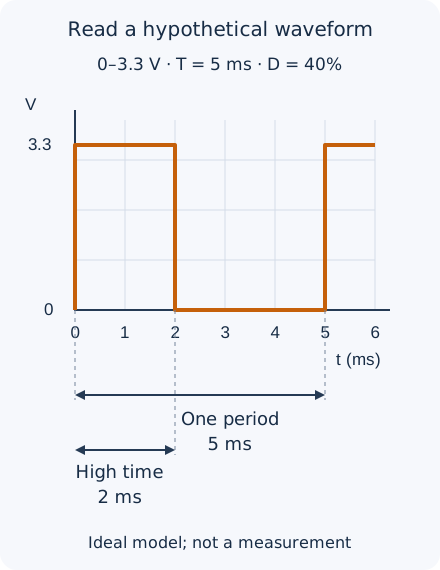
T = 5 ms = 0.005 s
f = 1 / T = 200 Hz
Duty = high time / period × 100
Duty = 2 / 5 × 100 = 40%
Hertz counts cycles per second. Duty cycle is the high-time fraction, rather than a voltage unit. At one millisecond per horizontal division, a period occupies five divisions and the high section occupies two. At one volt per vertical division, the levels differ by 3.3 divisions. Identify the zero-voltage reference too: the bottom of the screen is not necessarily zero volts. Our PWM and frequency lesson explains an application of this timing ratio.
What does a logic analyzer retain?
A logic analyzer's digital input classifies voltage as low or high according to its detection thresholds. A threshold is a decision boundary; some inputs use different boundaries for switching high and switching back low. These boundaries and the permitted input-voltage range depend on the instrument. A displayed one is not a precise 3.3-volt measurement, nor does it prove that the actual receiving device recognized the same state.
With several data and clock lines, the analyzer records their transitions and a suitable decoder interprets them as messages. A clock coordinates when data is read. Incorrect protocol, speed or polarity settings can produce misleading decoded text, so inspect the transitions before trusting the message. Saleae's input settings guide illustrates model-dependent thresholds and sample-rate options; it is not a specification for every analyzer.
A pulse might cross the analyzer's threshold yet fail to reach the voltage required by the receiving component. Its edge might also cross a boundary several times. An oscilloscope helps inspect voltage shape. Conversely, many digital channels and a long capture can make message sequencing easier to understand. Mixed instruments provide both capabilities. Choose a measurement according to the question and input specifications, rather than the name on the enclosure.
Separate sample rate, bandwidth and memory
A digital oscilloscope reads voltage at separate instants; each reading is a sample. Sample rate counts samples per second. At a hypothetical one million samples per second, successive samples are one microsecond apart. A microsecond is one millionth of a second. A shorter pulse may fit between samples and disappear from the record. Joining recorded points cannot restore an unobserved event.
Bandwidth concerns how the analog input path and probe pass rapid changes. A slow input can round an edge even when many samples are stored. A waveform repeating at 200 hertz can still have very fast edges, so repetition frequency alone is insufficient for choosing an instrument. The required rate depends on the narrowest event of interest and the instrument's behavior. “Twice the frequency” is not a universal recipe for observing pulses and edge shape.
Memory limits capture length. If one channel stores exactly one million samples at one million samples per second, the record lasts approximately one second. Increasing the rate tenfold with the same number of samples reduces it to one tenth of a second. That arithmetic describes simple continuous acquisition. Compression, active channels and acquisition modes can alter the practical relationship. Saleae's sample-rate guide discusses matching acquisition settings to signals and active channels.
How does a trigger find the event?
A trigger condition establishes a capture's time reference: for example, channel one crossing 1.5 volts upwards in our hypothetical waveform. The instrument may sample continuously and retain data from before and after that condition. A trigger therefore need not start all sampling. Suitable triggering steadies a repeating display; a unique fault needs a single acquisition and enough useful pre-event history.
With the wrong trigger source or level, an instrument may wait indefinitely or show an unsynchronized picture in automatic mode. First match the source, edge direction and level to the expected signal. A display reconstructed across multiple repetitions is insufficient evidence of a unique fault. Tektronix's XYZs primer explains vertical, horizontal and trigger systems separately.
The measurement connection becomes part of the circuit
A probe connects a circuit point to the input and can change circuit behavior through its resistance and capacitance. With a switchable attenuating probe, its setting and the channel's displayed attenuation must match the instructions for that combination. A mismatch between 1× and 10× can produce a voltage reading with the wrong scale factor. Adjusting probe compensation with the instrument's reference output tunes its response; it does not replace full instrument calibration or establish the accuracy of every measurement.
A long ground lead can distort the observation of fast edges. An appropriately short reference connection helps, but choosing the reference point comes first. On many bench oscilloscopes, input common and channel grounds connect to protective earth and to one another. Attaching a ground clip to an arbitrary circuit node can create a short circuit. Do not disconnect the instrument's protective earth. This lesson does not authorize mains measurements or floating-node measurements using an ordinary probe; those require suitably rated equipment and specialist methods. See Tektronix's probe primer and note on earth-referenced measurements.
A useful sequence for a low-voltage investigation
First write down the question and expected quantity: amplitude, period or ordering between two lines? Establish the circuit reference and permitted instrument inputs from their documentation. Once a suitable connection has been chosen, set probe attenuation, coupling and scales. DC coupling passes the steady component and changes; AC coupling removes the steady component and can distort slow pulses. DC coupling is a useful starting point for understanding our zero-to-3.3-volt example.
Then set the trigger and record length, and note the actual sample rate in that configuration. Retain the capture, settings and test conditions together. When investigating an unexpected shape, change one factor at a time, such as the probe connection, scale or circuit conditions. Our accuracy and calibration lesson explains why displayed digits do not establish correctness.
Exercise: what does the record establish?
A hypothetical waveform stays high for one millisecond and repeats every five milliseconds. Calculate frequency and duty cycle. If an analyzer records high, do you know the exact voltage? With samples only at zero, 3 and 6 milliseconds, must a pulse occurring between 1 and 2 milliseconds be visible?
Answer and reasoning
Frequency is 200 hertz and duty cycle is 20 percent. High reports that analyzer input's decision under the capture settings; it establishes neither precise voltage nor the receiving component's decision. Samples at zero, 3 and 6 milliseconds can all fall outside the pulse between 1 and 2 milliseconds. Its absence from those samples therefore does not prove its absence from the circuit.
The drawings and numerical examples are models and calculations. This lesson explains measurement concepts and selects no exact product for purchase. Specifications, compatibility and current availability of any product require a separate check.
Question and answer article
Ask your technical question
Questions and answers are published after moderation. Authors can see their own pending drafts.
No confirmed questions have been registered for this article yet.