Sensor sampling: why a fast change can look slow
See aliasing through two waveforms with identical samples, then separate conversion rate, display rate and filtering before the ADC.
Contents
When an input changes faster than a system can sample it faithfully, recorded data can show a plausible but much slower variation. This ambiguity is aliasing. Smoothing the chart is insufficient: input bandwidth, the actual conversion rate and filtering before sampling must be chosen together.
Imagine a sensor on a structure converting vibration into voltage. Software reads it several times per second and displays a calm trace. That trace alone does not establish that the structure vibrates slowly. We first need to understand what can be lost between recorded points.
Sample, sample rate and signal frequency
A sample is a value at an instant. An analog-to-digital converter, or ADC, reads a continuous input at separate instants and turns it into numbers. Sample rate counts these readings per second and is written f_s. Signal frequency counts the waveform’s cycles per second, measured in hertz. The two counts need not be equal.
Uniform sampling means equally spaced sampling instants. At 40 samples per second, the interval is 1 / 40 = 0.025 s = 25 ms. This is different from refreshing a display 40 times per second: a display may show the same result repeatedly.
Worked example: how 30 Hz can look like 10 Hz
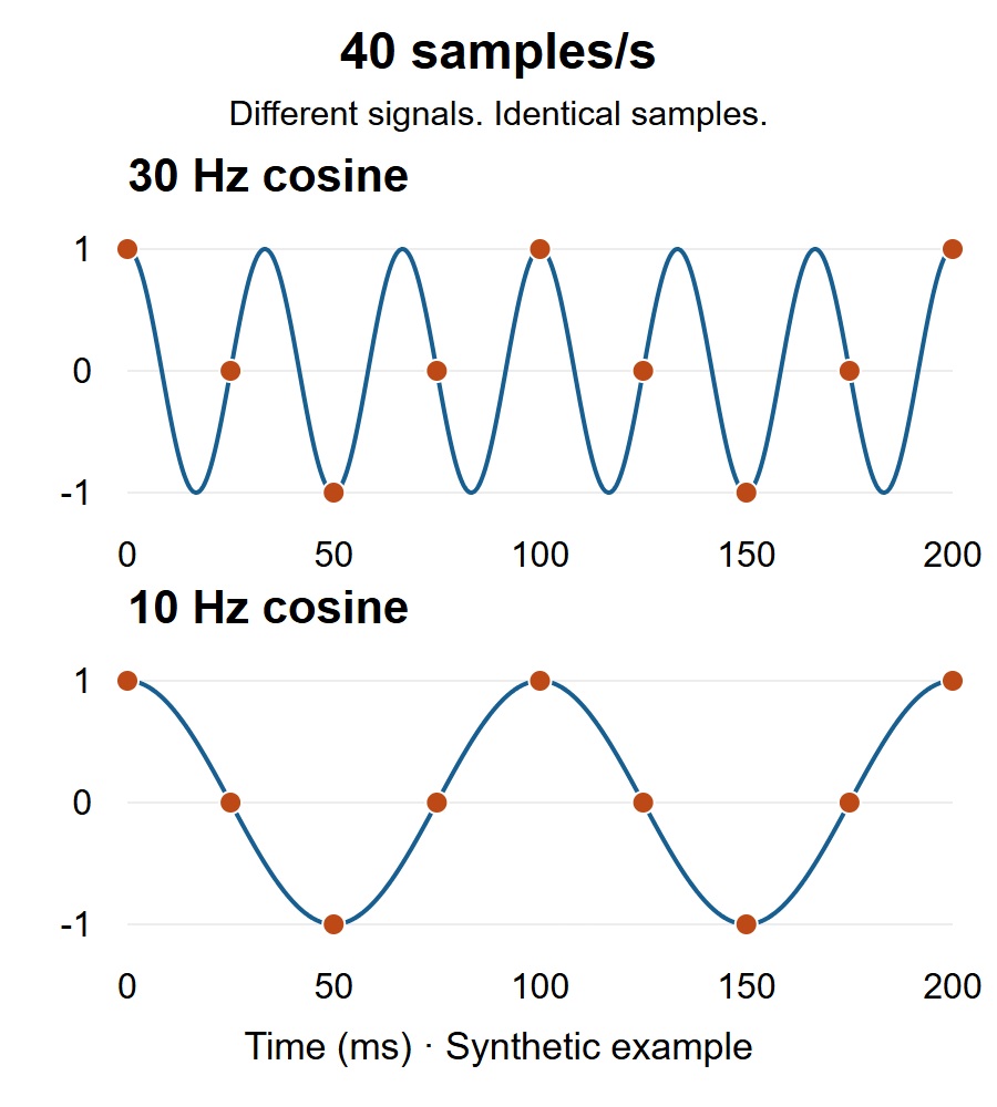
Take two ideal cosines with unit amplitude and the same initial phase, without noise or conversion error. One completes 30 cycles per second and the other completes 10. If we inspect them only at t = n / 40, their values are identical for every integer n:
t[n] = n / 40 seconds
x30[n] = cos(2*pi*30*n/40)
x10[n] = cos(2*pi*10*n/40)
x30[n] = x10[n]
At zero, 25, 50, 75 and 100 milliseconds, for example, both give 1, 0, −1, 0 and 1. A computer calculation may represent the zeros with tiny rounding errors. Between those instants, the 30 Hz waveform has followed a different path. The recorded points alone therefore cannot tell us which waveform was actually present.
In this example, the lower-band alias is |30 − 40| = 10 Hz. This calculation concerns two specified cosines, rather than a general signal-identification method. More decimal places or amplitude calibration cannot resolve the time-domain ambiguity. Accuracy and resolution address a different question.
Nyquist: why exactly twice is a poor design target
For ideal uniform sampling of a real, low-pass input, its frequency content must be limited to below half the sample rate. That half-rate is the Nyquist frequency: 20 Hz for our 40 samples/s example. The 30 Hz input lies outside it. Analog Devices’ explanation describes how out-of-band components fold into the lower band.
The exact boundary is also sensitive to phase. A 20 Hz sine sampled at 40 samples/s can have every recorded value equal to zero for an appropriate starting phase. Real filters also lack an instantaneous cutoff. Avoid choosing a rate merely equal to twice the highest desired frequency: allow room for the filter transition and device limitations. The ADC performance guide explains the practical filter limitation. This lesson concerns low-pass inputs; deliberate bandpass sampling in radio involves different design assumptions.
Where does the filter belong?
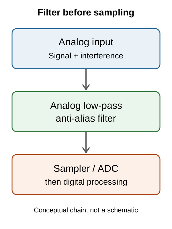
A low-pass filter passes slower variations while attenuating faster components. Anti-alias filtering must precede the stage where the ambiguity is introduced. A desired signal can be slow while faster electrical interference is added to it. NI’s guide explains why the input spectrum must be limited.
Once the identical points above have been recorded, an average or EMA cannot decide which of the two inputs produced them. Such filters remain useful for some noise, but cannot replace filtering before sampling. Our sensor-data filtering lesson examines their uses and delays separately.
Reading a digital sensor register is not necessarily a new sample
Some sensors contain an ADC and internal filters. Reading a register faster may simply return the previous result again. Check the actual model’s conversion rate, output data rate, data-ready indication and settling time. There is no universal rate or register setting for every sensor.
Discarding samples to reduce a high-rate data stream creates another rate-reduction stage. Unwanted frequency content must be limited before that stage too. A digital filter before downsampling can perform that job; MathWorks’ decimation documentation explains the ordering. This is different from trying to repair aliasing already introduced at the ADC.
Investigating a suspicious measurement
Retain raw values and actual sampling timestamps. Establish whether a programmed rate refers to fresh conversions or display refreshes. In a controlled experiment within the equipment’s limits, change the sampling rate and observe whether a suspicious component moves. Movement can be a clue, rather than proof of a single cause. The comparison instrument’s bandwidth and acquisition settings also matter; the oscilloscope and logic-analyzer lesson explains that distinction.
For an exercise without a circuit, open the sample table. The accompanying Python program only calculates values and writes a CSV; it does not connect to a device. It was run with Python 3.12.
Exercise: what lower-band alias does a 35 Hz waveform produce at 40 samples/s? In this model, |35 − 40| = 5 Hz. Start prevention with the requirement: if you need to retain the actual 35 Hz component, removing it with a low-pass filter is not a solution. The sampling rate and input path must be designed to preserve it.
Question and answer article
Ask your technical question
Questions and answers are published after moderation. Authors can see their own pending drafts.
No confirmed questions have been registered for this article yet.